BERT_topic_analysis

运行 Colab

Connect to kaggle

1
2
3
4
5
6
7
8
!pip install --user kaggle
!mkdir /root/.kaggle

!mv /content/kaggle.json /root/.kaggle/kaggle.json

!kaggle competitions download -c commonlitreadabilityprize

!ls
1
2
3
4
5
6
import os

for filename in os.listdir('.'):
if filename.endswith('.zip'):
os.system("unzip {}".format(filename))
os.system("rm {}".format(filename))

Visualization with Bokeh

1
2
3
4
5
6
7
8
9
!pip install --upgrade pip
!pip install --upgrade numpy
!pip install --upgrade sentence_transformers
!conda install -c conda-forge hdbscan --y
!pip install bokeh
!pip install --upgrade bertopic[visualization]

# !pip uninstall numpy
# !pip install numpy
1
2
3
4
5
6
7
8
9
10
11
12
13
14
15
16
17
18
19
20
21
22
23
from bertopic import BERTopic
import pandas as pd
from sentence_transformers import SentenceTransformer
import sklearn.manifold
import umap
import numpy as np
import pandas as pd
import random
from nltk.corpus import stopwords

random.seed(42)

from bokeh.io import output_file, show
from bokeh.models import ColumnDataSource, HoverTool, LinearColorMapper
from bokeh.palettes import plasma, d3, Turbo256
from bokeh.plotting import figure
from bokeh.transform import transform
import bokeh.io
bokeh.io.output_notebook()

import bokeh.plotting as bpl
import bokeh.models as bmo
bpl.output_notebook()

读取数据

1
2
3
4
5
6
7
8
9
10
11
12
test = pd.read_csv('test.csv')
train = pd.read_csv('train.csv')

train['set'] = 'train'
test['set'] = 'test'

combined = pd.concat([train, test], ignore_index=True)
combined.target.fillna(3, inplace=True)

texts = combined.excerpt.values.tolist()
targets = combined.target.values.tolist()
sets = combined.set.values.tolist()

文本处理(可选)

1
2
3
4
5
6
7
8
9
10
11
12
13
14
15
16
17
18
19
20
21
22
23
24
25
26
27
28
29
30
31
32
33
34
35
36
37
38
39
# def preprocess_tweet_data(data,name):
# # Lowering the case of the words in the sentences
# data[name]=data[name].str.lower()
# # Code to remove the Hashtags from the text
# data[name]=data[name].apply(lambda x:re.sub(r'\B#\S+','',x))
# # Code to remove the links from the text
# data[name]=data[name].apply(lambda x:re.sub(r"http\S+", "", x))
# # Code to remove the Special characters from the text
# data[name]=data[name].apply(lambda x:' '.join(re.findall(r'\w+', x)))
# # Code to substitute the multiple spaces with single spaces
# data[name]=data[name].apply(lambda x:re.sub(r'\s+', ' ', x, flags=re.I))
# # Code to remove all the single characters in the text
# data[name]=data[name].apply(lambda x:re.sub(r'\s+[a-zA-Z]\s+', '', x))
# # Remove the twitter handlers
# data[name]=data[name].apply(lambda x:re.sub('@[^\s]+','',x))


def preprocess(data):
excerpt_processed=[]
for e in data['excerpt']:
# find alphabets
e = re.sub("[^a-zA-Z]", " ", e)
e = re.sub(r'\s+', ' ', e, flags=re.I)

# # convert to lower case
# e = e.lower()

# tokenize words
e = nltk.word_tokenize(e)
# remove stopwords
e = [word for word in e if not word.lower() in set(stopwords.words("english"))]
# lemmatization
lemma = nltk.WordNetLemmatizer()
e = [lemma.lemmatize(word) for word in e]
e=" ".join(e)

excerpt_processed.append(e)

return excerpt_processed

使用sentence bert计算文档向量

1
model = SentenceTransformer('stsb-distilbert-base')
id
1
embeddings = model.encode(texts)

降维 t-SNE 与 umap

  • t-SNE保留数据中局部结构。
  • UMAP保留数据中的本地和大部分全局结构。
  • UMAP比tSNE要快得多,当面对更多数据、更高维数据时
1
2
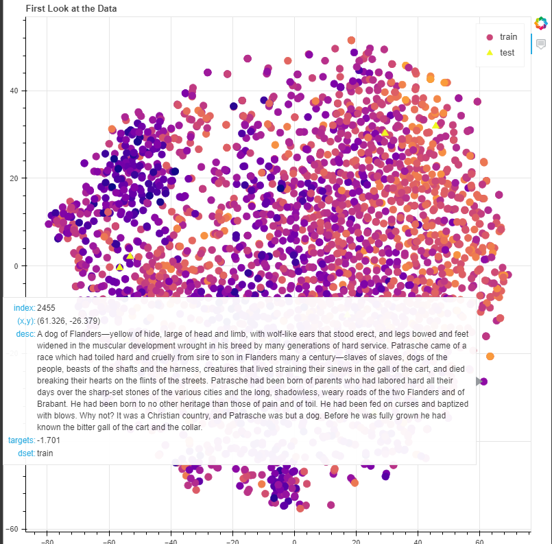
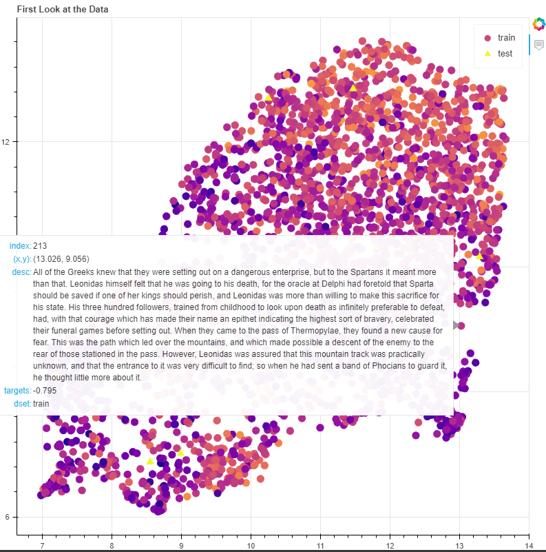
color_mapper = LinearColorMapper(palette='Plasma256', low=min(targets), high=max(targets))
out = sklearn.manifold.TSNE(n_components=2).fit_transform(embeddings)

绘制Boken。test set标签设置为3。

1
2
3
4
5
6
7
8
9
10
11
12
13
14
15
16
17
18
19
20
21
SETS = ['train', 'test']
MARKERS = ['circle', 'triangle']

list_x = out[:,0]
list_y = out[:,1]
desc = texts

source = ColumnDataSource(data=dict(x=list_x, y=list_y, desc=desc, targets=targets, dset=sets))
hover = HoverTool(tooltips=[
("index", "$index"),
("(x,y)", "(@x, @y)"),
('desc', '@desc'),
('targets', '@targets'),
('dset', '@dset')
])

p = figure(plot_width=800, plot_height=800, tools=[hover], title="First Look at the Data")
p.scatter('x', 'y', size=10, source=source, legend='dset', color={'field': 'targets', 'transform': color_mapper},
marker=bokeh.transform.factor_mark('dset', MARKERS, SETS),)

bpl.show(p)

1
2
umap_model = umap.UMAP(n_neighbors=15, n_components=2, metric='cosine')
out_umap = umap_model.fit_transform(embeddings)
1
2
3
4
5
6
7
8
9
10
11
12
13
14
15
16
17
18
19
20
21
SETS = ['train', 'test']
MARKERS = ['circle', 'triangle']

list_x = out_umap[:,0]
list_y = out_umap[:,1]
desc = texts

source = ColumnDataSource(data=dict(x=list_x, y=list_y, desc=desc, targets=targets, dset=sets))
hover = HoverTool(tooltips=[
("index", "$index"),
("(x,y)", "(@x, @y)"),
('desc', '@desc'),
('targets', '@targets'),
('dset', '@dset')
])

p = figure(plot_width=800, plot_height=800, tools=[hover], title="First Look at the Data")
p.scatter('x', 'y', size=10, source=source, legend='dset', color={'field': 'targets', 'transform': color_mapper},
marker=bokeh.transform.factor_mark('dset', MARKERS, SETS),)

bpl.show(p)

Kmeans 观察数据

1
2
3
4
5
from sklearn.decomposition import PCA
from sklearn.cluster import MiniBatchKMeans
from sklearn.metrics import silhouette_samples, silhouette_score
import matplotlib.pyplot as plt
import matplotlib.cm as cm
1
2
3
4
5
6
7
8
9
10
11
12
13
14
15
16
17
def find_optimal_clusters(data, max_k):
iters = range(2, max_k+1, 1)

sse = [] # 轮廓系数
for k in iters:
cluster = MiniBatchKMeans(n_clusters=k, init_size=256, batch_size=512, random_state=20).fit(data)
silhouette_avg = silhouette_score(data, cluster.labels_)
sse.append(silhouette_avg)
print('Fit {} clusters'.format(k))

f, ax = plt.subplots(1, 1)
ax.plot(iters, sse, marker='o')
ax.set_xlabel('Cluster Centers')
ax.set_xticks(iters)
ax.set_xticklabels(iters)
ax.set_ylabel('SSE')
ax.set_title('SSE by Cluster Center Plot')
colab
1
find_optimal_clusters(embeddings, 20)
1
clusters_2 = MiniBatchKMeans(n_clusters=2, init_size=256, batch_size=512, random_state=20).fit_predict(embeddings)
1
2
3
4
5
6
7
8
9
10
11
12
13
14
15
16
17
18
19
20
21
22
23
24
25
26
def plot_tsne_pca_umap(data, labels):
max_label = max(labels)+1
max_items = np.random.choice(range(data.shape[0]), size=2700, replace=False)

# reducer = umap.UMAP(n_components=2)
pca = PCA(n_components=2).fit_transform(data[max_items,:])
tsne = sklearn.manifold.TSNE(n_components=2).fit_transform(embeddings)
uma = umap.UMAP(n_components=2).fit_transform(embeddings)


idx = np.random.choice(range(pca.shape[0]), size=320, replace=False)
label_subset = labels[max_items]
label_subset = [cm.hsv(i/max_label) for i in label_subset[idx]]

f, ax = plt.subplots(1, 3, figsize=(14, 6))

ax[0].scatter(pca[idx, 0], pca[idx, 1], c=label_subset)
ax[0].set_title('PCA Cluster Plot')

ax[1].scatter(tsne[idx, 0], tsne[idx, 1], c=label_subset)
ax[1].set_title('TSNE Cluster Plot')

ax[2].scatter(uma[idx,0],uma[idx,1],c=label_subset)
ax[2].set_title('UMAP Cluster Plot')

plot_tsne_pca_umap(embeddings, clusters_2)

Topic

BERT topic

BERTopic依赖于句子嵌入和聚类算法,以及降维,生成文档主题簇。

1
2
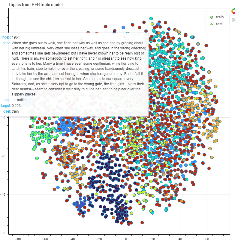
model = BERTopic(language="english", min_topic_size=20)
topics, probs = model.fit_transform(texts)
1
2
3
4
5
6
7
8
topic_words = ['-1: outlier']
for i in range(len(set(topics))-1):
tpc = model.get_topic(i)[:8]
words = [x[0] for x in tpc]
tw = ' '.join([str(i) + ':'] + words)
topic_words.append(tw)

exp_topics = [topic_words[x+1] for x in topics]
1
len(set(topics))
1
2
3
4
5
6
7
8
9
10
11
12
13
14
15
16
17
18
19
20
21
22
23
24
25
26
clrs = random.sample(Turbo256, len(set(topics)))
color_map = bmo.CategoricalColorMapper(factors=topic_words, palette=clrs)

list_x = out[:,0]
list_y = out[:,1]
desc = texts

source = ColumnDataSource(data=dict(x=list_x, y=list_y, desc=desc, topic=exp_topics, target=targets, dset=sets,))
hover = HoverTool(tooltips=[
("index", "$index"),
('desc', '@desc'),
('topic', '@topic'),
('target', '@target'),
('dset', '@dset'),
])

p = figure(plot_width=800, plot_height=800, tools=[hover], title="Topics from BERTopic model")
p.scatter('x', 'y', size=10, source=source,
fill_color=transform('topic', color_map),
marker=bokeh.transform.factor_mark('dset', MARKERS, SETS),
legend='dset'
)
# p.legend.location = "top_left"
# p.legend.click_policy="hide"

bokeh.plotting.show(p)

1
2
3
4
5
6
7
8
9
10
11
12
topic_df = model.get_topic_freq()

def get_keywords(i):
if i == -1: return 'outlier'
tpc = model.get_topic(i)[:8]
words = [x[0] for x in tpc]
tw = ' '.join(words)
return tw

topic_df['keywords'] = topic_df['Topic'].apply(get_keywords)

topic_df
1
model.get_topic(0)
1
model.visualize_topics()
1
# model.visualize_distribution(probs)

Classic LDA

id
1
import os
1
!pip install -Uqq gensim==3.8.3
1
2
3
4
5
6
# import os       #importing os to set environment variable
# def install_java():
# !apt-get install -y openjdk-8-jdk-headless -qq > /dev/null #install openjdk
# os.environ["JAVA_HOME"] = "/usr/lib/jvm/java-8-openjdk-amd64" #set environment variable
# !java -version #check java version
# install_java()
1
2
!wget -q http://mallet.cs.umass.edu/dist/mallet-2.0.8.zip
!unzip -qq mallet-2.0.8.zip
1
2
os.environ['MALLET_HOME'] = '/content/mallet-2.0.8'
mallet_path = '/content/mallet-2.0.8/bin/mallet' # you should NOT need to change this
1
2
3
4
5
6
7
8
9
10
11
12
13
14
15
16
import gensim
import gensim.corpora as corpora
from gensim.utils import simple_preprocess
from gensim.models.wrappers import LdaMallet
from gensim.models.coherencemodel import CoherenceModel
from gensim import similarities

import os.path
import re
import glob

import nltk
nltk.download('stopwords')

from nltk.tokenize import RegexpTokenizer
from nltk.corpus import stopwords
1
2
3
4
5
6
7
8
9
10
11
12
13
14
15
16
17
18
19
20
21
22
23
24
25
26
27
28
29
30
31
32
33
34
35
def preprocess_data(doc_set,extra_stopwords = {}):
# adapted from https://www.datacamp.com/community/tutorials/discovering-hidden-topics-python
# replace all newlines or multiple sequences of spaces with a standard space
doc_set = [re.sub('\s+', ' ', doc) for doc in doc_set]
# initialize regex tokenizer
tokenizer = RegexpTokenizer(r'\w+')
# create English stop words list
en_stop = set(stopwords.words('english'))
# add any extra stopwords
if (len(extra_stopwords) > 0):
en_stop = en_stop.union(extra_stopwords)

# list for tokenized documents in loop
texts = []
# loop through document list
for i in doc_set:
# clean and tokenize document string
raw = i.lower()
tokens = tokenizer.tokenize(raw)
# remove stop words from tokens
stopped_tokens = [i for i in tokens if not i in en_stop]
# add tokens to list
texts.append(stopped_tokens)
return texts

def prepare_corpus(doc_clean):
# adapted from https://www.datacamp.com/community/tutorials/discovering-hidden-topics-python
# Creating the term dictionary of our courpus, where every unique term is assigned an index. dictionary = corpora.Dictionary(doc_clean)
dictionary = corpora.Dictionary(doc_clean)

dictionary.filter_extremes(no_below=5, no_above=0.5)
# Converting list of documents (corpus) into Document Term Matrix using dictionary prepared above.
doc_term_matrix = [dictionary.doc2bow(doc) for doc in doc_clean]
# generate LDA model
return dictionary,doc_term_matrix
1
2
doc_clean = preprocess_data(texts,{})
dictionary, doc_term_matrix = prepare_corpus(doc_clean)
1
2
number_of_topics=30 # adjust this to alter the number of topics
words=10 #adjust this to alter the number of words output for the topic below
1
ldamallet = LdaMallet(mallet_path, corpus=doc_term_matrix, num_topics=number_of_topics, id2word=dictionary, alpha=10)
1
2
3
4
5
6
7
8
9
# topic_words = ldamallet.show_topics(num_topics=number_of_topics,num_words=5)
# topic_words = [x[1] for x in topic_words]

topic_words = []
for i in range(number_of_topics):
tpc = ldamallet.show_topic(i, topn=7, num_words=None)
words = [x[0] for x in tpc]
tw = ' '.join([str(i) + ':'] + words)
topic_words.append(tw)
1
topic_words
1
2
3
4
5
6
7
8
9
10
11
12
# show result
topics_docs = list()
for m in ldamallet[doc_term_matrix[:1000]]:
topics_docs.append(m)

x = np.array(topics_docs[:1000])
y = np.delete(x,0,axis=2)
y = y.squeeze()

best_topics = np.argmax(y, axis=1) # 结果是一个分布
topics = list(best_topics)
topics = [topic_words[x] for x in topics]
1
2
3
4
5
6
7
8
9
10
11
12
13
14
15
16
17
18
19
20
21
22
23
clrs = random.sample(Turbo256, number_of_topics)
color_map = bmo.CategoricalColorMapper(factors=topic_words, palette=clrs)

list_x = out[:,0]
list_y = out[:,1]
desc = texts

source = ColumnDataSource(data=dict(x=list_x, y=list_y, desc=desc, topic=topics))
hover = HoverTool(tooltips=[
("index", "$index"),
('desc', '@desc'),
('topic', '@topic')
])

p = figure(plot_width=1200, plot_height=600, tools=[hover], title="Test")
p.circle('x', 'y', size=10, source=source,
fill_color=transform('topic', color_map),
# legend='topic'
)
# p.legend.location = "top_left"
# p.legend.click_policy="hide"

bpl.show(p)

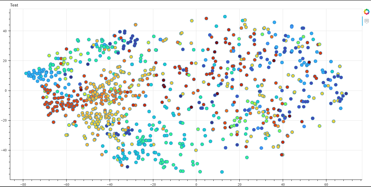
看上面的图表,由LDA重新识别的主题内文档不一定相互接近。 与BERTopic是互补的,可以得到不同的主题表示。

Bertopic在短文本这类可能只有一个主题的文本中表现较好,而LDA可以更好地处理主题组合较多的文本。 两者可以互补,因此尝试两者都有意义。

这和两者的原理是相关的,Bertopic是空间距离的聚类,LDA是统计层面的共现规律分析。

1
2
# pyLDAvis可视化
!pip install -Uqq pyLDAvis==2.1.2
1
gensimmodel = gensim.models.wrappers.ldamallet.malletmodel2ldamodel(ldamallet)
1
2
3
4
5
6
import pyLDAvis
import pyLDAvis.gensim

pyLDAvis.enable_notebook()
p = pyLDAvis.gensim.prepare(gensimmodel, doc_term_matrix, dictionary)
p

ref: https://skok.ai/2021/05/27/Topic-Models-Introduction.html

BERTopic 详解

BERTopic,利用BERT嵌入和c-TF-IDF来创建密集的集群,使话题易于解释,同时在话题描述中保留重要词汇。其核心步骤主要是做三件事:

  • 用基于BERT的Sentence Transformers提取语句嵌入
  • 通过UMAP和HDBSCAN,将文档嵌入进行聚类,语义相近的语句将聚集成簇群
  • 用c-TF-IDF提取主题词

c-TF-IDF就是将一个主题下的所有文档连接在一起成为一个文档,在主题间计算TF-IDF的方法。

1
2
3
4
5
6
7
8
9
10
11
12
13
import numpy as np
import pandas as pd
import jieba
import umap
import hdbscan
from sentence_transformers import SentenceTransformer
from sklearn.feature_extraction.text import CountVectorizer
from sklearn.metrics.pairwise import cosine_similarity
from tqdm import tqdm
import matplotlib.pyplot as plt

# import sys
# sys.setrecursionlimit(1000000)
1
2
3
4
5
6
7
8
9
10
11
12
13
14
15
16
17
18
19
20
21
22
23
24
25
26
27
28
29
30
31
32
33
34
35
36
37
38
39
40
41
42
43
44
# model = SentenceTransformer(r'my_pretrained_chinese_embeddings')
# embeddings = model.encode(data['review'].tolist(), show_progress_bar=True)

#### 降维
umap_embeddings = umap.UMAP(
n_neighbors=25,
n_components=10,
min_dist=0.00,
metric='cosine',
random_state=2020).fit_transform(embeddings)


#### 聚类
# 使用HDBSCAN来寻找高密簇
cluster = hdbscan.HDBSCAN(
min_cluster_size=30,
metric='euclidean',
cluster_selection_method='eom',
prediction_data=True).fit(umap_embeddings)


#### c-TF-IDF
def c_tf_idf(documents, m, ngram_range=(1, 1)):
my_stopwords = [i.strip() for i in open('stop_words_zh.txt',encoding='utf-8').readlines()]

count = CountVectorizer(
ngram_range=ngram_range,
stop_words= my_stopwords).fit(documents)

t = count.transform(documents).toarray()

w = t.sum(axis=1)
tf = np.divide(t.T, w)

sum_t = t.sum(axis=0)
idf = np.log(np.divide(m, sum_t)).reshape(-1, 1)

tf_idf = np.multiply(tf, idf)

return tf_idf, count


#### 主题归并
# 通过比较主题之间的c-TF-IDF向量,合并最相似的向量,最后重新计算c-TF-IDF向量来更新主题的表示

本博客所有文章除特别声明外,均采用 CC BY-SA 4.0 协议 ,转载请注明出处!