Practical BERT

BERT类模型，基本使用流程：1. Further pretrain. 2. single-task or multi-task finetuning. 3. inference

Further pretraining一般使用任务数据进行，也可以使用与任务数据相似的 in-domain 数据，或者使用数据量更大但是和任务数据不那么相关的数据进行。

一般而言使用任务数据的效果会好一些。但是数据量不足，且能找到与任务数据相似的 in-domain 数据，也可以稳定提高模型效果。（ref）

Transformer Representations

Transformer 不同的层捕获不同层次的表示。比如、下层是表层（字、词）特征，中层是句法特征，上层是语义特征。

如图为不同的embedding表示，输入BiLSTM进行NER任务的结果对比。

BERT的不同层编码的信息非常不同，因此适当的池化策略，应该根据不同应用而改变，因为不同的层编码不同的信息。

Hugging Face的BERT模型一般输出为：

• last hidden state (batch size, seq len, hidden size) which is the sequence of hidden states at the output of the last layer.
• pooler output (batch size, hidden size) - Last layer hidden-state of the first token of the sequence
• hidden states (n layers, batch size, seq len, hidden size) - Hidden states for all layers and for all ids.

Pooler output

pooler output，最后一层的[CLS] token的hidden state，接一个Linear layer 和一个 Tanh activation function的结果。预训练时，作为next sentence prediction (classification) objective的计算结果。

在config中可以设置 pooling layer 为 False，不输出这一结果。

...
max_seq_length = 256
_pretrained_model = 'roberta-base'

config = AutoConfig.from_pretrained(_pretrained_model)
model = AutoModel.from_pretrained(_pretrained_model, config=config)
tokenizer = AutoTokenizer.from_pretrained(_pretrained_model)

clear_output()

features = tokenizer.batch_encode_plus(
    train_text,
    add_special_tokens=True,
    padding='max_length',
    max_length=max_seq_length,
    truncation=True,
    return_tensors='pt',
    return_attention_mask=True
)

outputs = model(features['input_ids'], features['attention_mask'])

pooler_output = outputs[1]

logits = nn.Linear(config.hidden_size, 1)(pooler_output) # regression head
...

More than last hidden state

最后一层输出的 hidden state，[batch, maxlen, hidden_state]。其中[batch, 1, hidden_state]对应 [CLS]。

CLS Embeddings

with torch.no_grad():
    outputs = model(features['input_ids'], features['attention_mask'])
last_hidden_state = outputs[0]

cls_embeddings = last_hidden_state[:, 0]

可以处理简单的下游任务，将cls_embeddings作为整个序列的一个简单表示。

Mean Pooling

features = tokenizer.batch_encode_plus(
    train_text,
    add_special_tokens=True,
    padding='max_length',
    max_length=max_seq_length,
    truncation=True,
    return_tensors='pt',
    return_attention_mask=True
)
attention_mask = features['attention_mask']
...

# Step 1: Expand Attention Mask from [batch_size, max_len] to [batch_size, max_len, hidden_size].
input_mask_expanded = attention_mask.unsqueeze(-1).expand(last_hidden_state.size()).float()
# Step 2: Sum Embeddings along max_len axis so now we have [batch_size, hidden_size]
sum_embeddings = torch.sum(last_hidden_state * input_mask_expanded, 1)
# Step 3: Sum Mask along max_len axis.
sum_mask = input_mask_expanded.sum(1)
sum_mask = torch.clamp(sum_mask, min=1e-9)
# Step 4: Take Average.
mean_embeddings = sum_embeddings / sum_mask

logits = nn.Linear(config.hidden_size, 1)(mean_embeddings) # regression head

在max len维度，进行平均。

Max Pooling

在max len维度，进行max pooling

# input_mask_expanded = attention_mask.unsqueeze(-1).expand(last_hidden_state.size()).float()
# last_hidden_state[input_mask_expanded == 0] = -1e9  # Set padding tokens to large negative value
max_embeddings = torch.max(last_hidden_state, 1)[0]

Mean-Max Pooling (Head)

input_mask_expanded = attention_mask.unsqueeze(-1).expand(last_hidden_state.size()).float()
sum_embeddings = torch.sum(last_hidden_state * input_mask_expanded, 1)
sum_mask = input_mask_expanded.sum(1)
sum_mask = torch.clamp(sum_mask, min=1e-9)
mean_embeddings = sum_embeddings / sum_mask

max_pooling_embeddings, _ = torch.max(last_hidden_state, 1)

cls_embeddings = last_hidden_state[:, 0]

mean_max_embeddings = torch.cat((mean_pooling_embeddings, max_pooling_embeddings, cls_embeddings), 1)
logits = nn.Linear(config.hidden_size * 3, 1)(mean_max_embeddings) # 3 hidden size

Conv-1D Pooling

# first define layers
cnn1 = nn.Conv1d(768, 256, kernel_size=2, padding=1)
cnn2 = nn.Conv1d(256, 1, kernel_size=2, padding=1)

last_hidden_state = last_hidden_state.permute(0, 2, 1) # (batch size, hidden size, seq len)
cnn_embeddings = F.relu(cnn1(last_hidden_state))
cnn_embeddings = cnn2(cnn_embeddings)
logits, _ = torch.max(cnn_embeddings, 2)  # max pooling in Length dim

More than Hidden States Output

embeddings 与 每一层的输出集合，(n_layers, batch_size, sequence_length, hidden_size)。

...
max_seq_length = 256
_pretrained_model = 'roberta-base'

config = AutoConfig.from_pretrained(_pretrained_model)
# 设置输出选项
config.update({'output_hidden_states':True})

model = AutoModel.from_pretrained(_pretrained_model, config=config)
tokenizer = AutoTokenizer.from_pretrained(_pretrained_model)
clear_output()
features = tokenizer.batch_encode_plus(
    train_text,
    add_special_tokens=True,
    padding='max_length',
    max_length=max_seq_length,
    truncation=True,
    return_tensors='pt',
    return_attention_mask=True
)

with torch.no_grad():
    outputs = model(features['input_ids'], features['attention_mask'])
all_hidden_states = torch.stack(outputs[2])

CLS Layer Embeddings

倒数第二层示例

layer_index = 11 # second to last hidden layer
cls_embeddings = all_hidden_states[layer_index, :, 0] # 13 layers (embedding + num of blocks)

logits = nn.Linear(config.hidden_size, 1)(cls_embeddings) # regression head

GitHub的bert-as-service 项目，就是默认取得倒数第二层的输出。更好地表示语义，而不被MLM任务和NSP任务影响太多。

Concatenate Pooling

最后四层 CLS concat.

all_hidden_states = torch.stack(outputs[2])

concatenate_pooling = torch.cat(
    (all_hidden_states[-1], all_hidden_states[-2], all_hidden_states[-3], all_hidden_states[-4]), -1
)
concatenate_pooling = concatenate_pooling[:, 0]  # first token

logits = nn.Linear(config.hidden_size*4, 1)(concatenate_pooling)

Weighted Layer Pooling

基于一个intuition，fine-tuning时，最容易被训练的应该是middle layer的表达，因为顶层是专门用于 language modeling pre-train 任务的。所以只使用顶层的输出进行下游任务，会限制模型的效果。（没有实证，一个假设）

class WeightedLayerPooling(nn.Module):
    def __init__(self, num_hidden_layers, layer_start: int = 4, layer_weights = None):
        super(WeightedLayerPooling, self).__init__()
        self.layer_start = layer_start
        self.num_hidden_layers = num_hidden_layers
        self.layer_weights = layer_weights if layer_weights is not None \
            else nn.Parameter(
                torch.tensor([1] * (num_hidden_layers+1 - layer_start), dtype=torch.float)
            )

    def forward(self, all_hidden_states):
        all_layer_embedding = all_hidden_states[self.layer_start:, :, :, :]
        weight_factor = self.layer_weights.unsqueeze(-1).unsqueeze(-1).unsqueeze(-1).expand(all_layer_embedding.size())
        weighted_average = (weight_factor*all_layer_embedding).sum(dim=0) / self.layer_weights.sum()
        return weighted_average
    
# 使用：最后四层的 CLS 表示，计算加权和
layer_start = 9
pooler = WeightedLayerPooling(
    config.num_hidden_layers, 
    layer_start=layer_start, layer_weights=None
)
weighted_pooling_embeddings = pooler(all_hidden_states)
weighted_pooling_embeddings = weighted_pooling_embeddings[:, 0]
logits = nn.Linear(config.hidden_size, 1)(weighted_pooling_embeddings)

LSTM/GRU Pooling

\[ o = h^L_{LSTM} =LSTM(h^i_{CLS}), i ∈ [1, L] \] CLS token输入LSTM，得到最终表示

class LSTMPooling(nn.Module):
    def __init__(self, num_layers, hidden_size, hiddendim_lstm):
        super(LSTMPooling, self).__init__()
        self.num_hidden_layers = num_layers
        self.hidden_size = hidden_size
        self.hiddendim_lstm = hiddendim_lstm
        self.lstm = nn.LSTM(self.hidden_size, self.hiddendim_lstm, batch_first=True)
        self.dropout = nn.Dropout(0.1)
    
    def forward(self, all_hidden_states):
        ## forward
        hidden_states = torch.stack([all_hidden_states[layer_i][:, 0].squeeze()
                                     for layer_i in range(1, self.num_hidden_layers+1)], dim=-1)
        hidden_states = hidden_states.view(-1, self.num_hidden_layers, self.hidden_size)
        out, _ = self.lstm(hidden_states, None)
        out = self.dropout(out[:, -1, :])
        return out

hiddendim_lstm = 256
pooler = LSTMPooling(config.num_hidden_layers, config.hidden_size, hiddendim_lstm)
lstm_pooling_embeddings = pooler(all_hidden_states)
logits = nn.Linear(hiddendim_lstm, 1)(lstm_pooling_embeddings) # regression head

Attention Pooling

dot-product attention： \[ o = W^T_{h} softmax(qh^T_{CLS})h_{CLS} \] \(W^T_{h}\) 和 \(q\)为可学习参数。

class AttentionPooling(nn.Module):
    def __init__(self, num_layers, hidden_size, hiddendim_fc):
        super(AttentionPooling, self).__init__()
        self.num_hidden_layers = num_layers
        self.hidden_size = hidden_size
        self.hiddendim_fc = hiddendim_fc
        self.dropout = nn.Dropout(0.1)

        q_t = np.random.normal(loc=0.0, scale=0.1, size=(1, self.hidden_size))
        self.q = nn.Parameter(torch.from_numpy(q_t)).float()
        w_ht = np.random.normal(loc=0.0, scale=0.1, size=(self.hidden_size, self.hiddendim_fc))
        self.w_h = nn.Parameter(torch.from_numpy(w_ht)).float()

    def forward(self, all_hidden_states):
        hidden_states = torch.stack([all_hidden_states[layer_i][:, 0].squeeze()
                                     for layer_i in range(1, self.num_hidden_layers+1)], dim=-1)
        hidden_states = hidden_states.view(-1, self.num_hidden_layers, self.hidden_size)
        out = self.attention(hidden_states)
        out = self.dropout(out)
        return out

    def attention(self, h):
        v = torch.matmul(self.q, h.transpose(-2, -1)).squeeze(1)
        v = F.softmax(v, -1)
        v_temp = torch.matmul(v.unsqueeze(1), h).transpose(-2, -1)
        v = torch.matmul(self.w_h.transpose(1, 0), v_temp).squeeze(2)
        return v

hiddendim_fc = 128
pooler = AttentionPooling(config.num_hidden_layers, config.hidden_size, hiddendim_fc)
attention_pooling_embeddings = pooler(all_hidden_states)
logits = nn.Linear(hiddendim_fc, 1)(attention_pooling_embeddings) # regression head

WKPooling

来自论文: SBERT-WK: A Sentence Embedding Method By Dissecting BERT-based Word Models

通过计算 每一层每个token的 alignment and novelty properties，得到每个token的 unified word representation。然后根据计算得到每个token 的 word importance ，加权求和得到一个 Sentence Embedding 表示。

计算中用到 QR分解，然而pytorch在GPU上计算QR很慢，所以转到CPU上计算，但是这依然很慢（相比于其他在GPU上的操作）。

class WKPooling(nn.Module):
    def __init__(self, layer_start: int = 4, context_window_size: int = 2):
        super(WKPooling, self).__init__()
        self.layer_start = layer_start
        self.context_window_size = context_window_size

    def forward(self, all_hidden_states):
        ft_all_layers = all_hidden_states
        org_device = ft_all_layers.device
        all_layer_embedding = ft_all_layers.transpose(1,0)
        all_layer_embedding = all_layer_embedding[:, self.layer_start:, :, :]  # Start from 4th layers output

        # torch.qr is slow on GPU (see https://github.com/pytorch/pytorch/issues/22573). So compute it on CPU until issue is fixed
        all_layer_embedding = all_layer_embedding.cpu()

        attention_mask = features['attention_mask'].cpu().numpy()
        unmask_num = np.array([sum(mask) for mask in attention_mask]) - 1  # Not considering the last item
        embedding = []

        # One sentence at a time
        for sent_index in range(len(unmask_num)):
            sentence_feature = all_layer_embedding[sent_index, :, :unmask_num[sent_index], :]
            one_sentence_embedding = []
            # Process each token
            for token_index in range(sentence_feature.shape[1]):
                token_feature = sentence_feature[:, token_index, :]
                # 'Unified Word Representation'
                token_embedding = self.unify_token(token_feature)
                one_sentence_embedding.append(token_embedding)

            ##features.update({'sentence_embedding': features['cls_token_embeddings']})

            one_sentence_embedding = torch.stack(one_sentence_embedding)
            sentence_embedding = self.unify_sentence(sentence_feature, one_sentence_embedding)
            embedding.append(sentence_embedding)

        output_vector = torch.stack(embedding).to(org_device)
        return output_vector

    def unify_token(self, token_feature):
        ## Unify Token Representation
        window_size = self.context_window_size

        alpha_alignment = torch.zeros(token_feature.size()[0], device=token_feature.device)
        alpha_novelty = torch.zeros(token_feature.size()[0], device=token_feature.device)

        for k in range(token_feature.size()[0]):
            left_window = token_feature[k - window_size:k, :]
            right_window = token_feature[k + 1:k + window_size + 1, :]
            window_matrix = torch.cat([left_window, right_window, token_feature[k, :][None, :]])
            Q, R = torch.qr(window_matrix.T)

            r = R[:, -1]
            alpha_alignment[k] = torch.mean(self.norm_vector(R[:-1, :-1], dim=0), dim=1).matmul(R[:-1, -1]) / torch.norm(r[:-1])
            alpha_alignment[k] = 1 / (alpha_alignment[k] * window_matrix.size()[0] * 2)
            alpha_novelty[k] = torch.abs(r[-1]) / torch.norm(r)

        # Sum Norm
        alpha_alignment = alpha_alignment / torch.sum(alpha_alignment)  # Normalization Choice
        alpha_novelty = alpha_novelty / torch.sum(alpha_novelty)

        alpha = alpha_novelty + alpha_alignment
        alpha = alpha / torch.sum(alpha)  # Normalize

        out_embedding = torch.mv(token_feature.t(), alpha)
        return out_embedding

    def norm_vector(self, vec, p=2, dim=0):
        ## Implements the normalize() function from sklearn
        vec_norm = torch.norm(vec, p=p, dim=dim)
        return vec.div(vec_norm.expand_as(vec))

    def unify_sentence(self, sentence_feature, one_sentence_embedding):
        ## Unify Sentence By Token Importance
        sent_len = one_sentence_embedding.size()[0]

        var_token = torch.zeros(sent_len, device=one_sentence_embedding.device)
        for token_index in range(sent_len):
            token_feature = sentence_feature[:, token_index, :]
            sim_map = self.cosine_similarity_torch(token_feature)
            var_token[token_index] = torch.var(sim_map.diagonal(-1))

        var_token = var_token / torch.sum(var_token)
        sentence_embedding = torch.mv(one_sentence_embedding.t(), var_token)

        return sentence_embedding
    
    def cosine_similarity_torch(self, x1, x2=None, eps=1e-8):
        x2 = x1 if x2 is None else x2
        w1 = x1.norm(p=2, dim=1, keepdim=True)
        w2 = w1 if x2 is x1 else x2.norm(p=2, dim=1, keepdim=True)
        return torch.mm(x1, x2.t()) / (w1 * w2.t()).clamp(min=eps)

pooler = WKPooling(layer_start=9)
wkpooling_embeddings = pooler(all_hidden_states)
logits = nn.Linear(config.hidden_size, 1)(wkpooling_embeddings) # regression head

Other methods

• Dense Pooling
• Word Weight (TF-IDF) Pooling
• Async Pooling
• Parallel / Heirarchical Aggregation

每个任务上，不同的方法表现有差异，应该根据情况选择使用不同的方法。

Few-Shot Stability

Fine-tuning Transformer models通常不稳定，收到超参数的影响大，不同的 random seed 也会导致不同的结果。

比如，在训练时，每个epoch中多进行evaluating，而不是在每个epoch之后evaluating，能够增加stability。

其他方法有：

• Debiasing Omission In BertADAM
• Re-Initializing Transformer Layers
• Utilizing Intermediate Layers
• Layer-wise Learning Rate Decay (LLRD)
• Mixout Regularization
• Pre-trained Weight Decay
• Stochastic Weight Averaging

通常不会一起用，可能会互向影响。方法各自提出的环境也不同。所以一般一两种方法的使用，能够提高模型性能。

Debiasing Omission In BERTAdam

rescaled_grad = clip(grad * rescale_grad, clip_gradient)
m = beta1 * m + (1 - beta1) * rescaled_grad
v = beta2 * v + (1 - beta2) * (rescaled_grad**2)
w = w - learning_rate * (m / (sqrt(v) + epsilon) + wd * w)

和标准Adam，差别在于 wd * w，增加了 weight decay。论文 Fixing Weight Decay Regularization in Adam 中提出的 AdamW，保留了 bias-correction terms （上面伪代码第2，3行），并且将 wd * w 加入 learning_rate 的影响。将下图中的紫色 weight decay 方法，改为绿色的部分。这样更新 x 时，weight decay 不会耦合参数 \(\beta\) 和 \(w_t\)（第7、8行），而是直接作用于 x（第12行）。

Debiasing Omission就是要保留 bias-correction terms 。在HuggingFace Transformers AdamW中设置 correct_bias parameter 为 True （default）。

lr = 2e-5
epsilon = 1e-6
weight_decay = 0.01

no_decay = ["bias", "LayerNorm.weight"]
optimizer_grouped_parameters = [{
    "params": [p for n, p in model.named_parameters() if not any(nd in n for nd in no_decay)],
    "weight_decay": weight_decay,
    "lr": lr},
    {"params": [p for n, p in model.named_parameters() if any(nd in n for nd in no_decay)],
    "weight_decay": 0.0,
    "lr": lr}
]

optimizer = AdamW(
    optimizer_grouped_parameters,
    lr=lr,
    eps=epsilon,
    correct_bias=True
)

Reinitializing Transformer Layers

来自计算机视觉的直觉，高层与预训练任务相关的层，可以重新训练。

比如，Reinitialize Pooler layer的参数

add_pooler = True
reinit_pooler = True

class Net(nn.Module):
    def __init__(self, config, _pretrained_model, add_pooler):
        super(Net, self).__init__()
        self.roberta = RobertaModel.from_pretrained(_pretrained_model, add_pooling_layer=add_pooler)
        self.classifier = RobertaClassificationHead(config)
        
    def forward(self, input_ids, attention_mask):
        outputs = self.roberta(input_ids, attention_mask=attention_mask,)
        sequence_output = outputs[0]
        logits = self.classifier(sequence_output)
        return logits
        
model = Net(config, _pretrained_model, add_pooler)

if reinit_pooler:
    print('Reinitializing Pooler Layer ...')
    encoder_temp = getattr(model, _model_type)
    encoder_temp.pooler.dense.weight.data.normal_(mean=0.0, std=encoder_temp.config.initializer_range)
    encoder_temp.pooler.dense.bias.data.zero_()
    for p in encoder_temp.pooler.parameters():
        p.requires_grad = True
    print('Done.!')

对 RoBERTa 的transformer layer进行 Reinitialize 。

RoBERTa 不同于 BERT 在于：

• 没有 next-sentence pretraining objective ，更改了超参，更大的 batch size 和learning rate
• 使用 byte level BPE 的 tokenizer
• 没有 token_type_ids，只需要 用 sep_token 分开不同 sentence。

检查是否被初始化：

for layer in model.roberta.encoder.layer[-reinit_layers:]:
    for module in layer.modules():
        if isinstance(module, nn.Linear):
            print(module.weight.data)

重新初始化

reinit_layers = 2
# TF version uses truncated_normal for initialization. This is Pytorch
if reinit_layers > 0:
    print(f'Reinitializing Last {reinit_layers} Layers ...')
    encoder_temp = getattr(model, _model_type)
    for layer in encoder_temp.encoder.layer[-reinit_layers:]:
        for module in layer.modules():
            if isinstance(module, nn.Linear):
                module.weight.data.normal_(mean=0.0, std=config.initializer_range)
                if module.bias is not None:
                    module.bias.data.zero_()
            elif isinstance(module, nn.Embedding):
                module.weight.data.normal_(mean=0.0, std=config.initializer_range)
                if module.padding_idx is not None:
                    module.weight.data[module.padding_idx].zero_()
            elif isinstance(module, nn.LayerNorm):
                module.bias.data.zero_()
                module.weight.data.fill_(1.0)
    print('Done.!')

另外 XLNet 实现方式有些不同 （Transformer-XL）：

reinit_layers = 2

if reinit_layers > 0:
    print(f'Reinitializing Last {reinit_layers} Layers ...')
    for layer in model.transformer.layer[-reinit_layers :]:
        for module in layer.modules():
            if isinstance(module, (nn.Linear, nn.Embedding)):
                module.weight.data.normal_(mean=0.0, std=model.transformer.config.initializer_range)
                if isinstance(module, nn.Linear) and module.bias is not None:
                    module.bias.data.zero_()
            elif isinstance(module, nn.LayerNorm):
                module.bias.data.zero_()
                module.weight.data.fill_(1.0)
            elif isinstance(module, XLNetRelativeAttention):
                for param in [
                    module.q,
                    module.k,
                    module.v,
                    module.o,
                    module.r,
                    module.r_r_bias,
                    module.r_s_bias,
                    module.r_w_bias,
                    module.seg_embed,
                ]:
                    param.data.normal_(mean=0.0, std=model.transformer.config.initializer_range)
    print('Done.!')

BART，是 seq2seq的结构，"BERT"作为encoder，"GPT"作为decoder（left-to-right）。采用了多样的噪声预训练方式。

• 随机token masking
• 随机token deletion
• 随机连续tokens替换为一个mask，或者直接插入一个mask
• 随机打乱文本sentence顺序
• 将文本序列连成环，随机选择文本开始位置

BART文本理解任务效果可以持平RoBERTa，且适合文本生成任务，而模型大小仅仅比BERT大10%。

reinit_layers = 2
_model_type = 'bart'
_pretrained_model = 'facebook/bart-base'
config = AutoConfig.from_pretrained(_pretrained_model)
config.update({'num_labels':1})
model = AutoModelForSequenceClassification.from_pretrained(_pretrained_model)

if reinit_layers > 0:
    print(f'Reinitializing Last {reinit_layers} Layers ...')
    for layer in model.model.decoder.layers[-reinit_layers :]:
        for module in layer.modules():
            model.model._init_weights(module)
    print('Done.!')

实验表明， Re-initialization 对 random seed 更 robust。不建议初始化超过6层的layer，不同任务需要实验找到最好的参数。

Utilizing Intermediate Layers

此部分就是本文第一节 Transformer Representations 的内容。

LLRD - Layerwise Learning Rate Decay

就是 low layer 通用信息，低学习率，top layer 任务相关信息，相对较高学习率。

一种方法是，每层有一个 decay rate

def get_optimizer_grouped_parameters(
    model, model_type, 
    learning_rate, weight_decay, 
    layerwise_learning_rate_decay
):
    no_decay = ["bias", "LayerNorm.weight"]
    
    # initialize lr for task specific layer
    optimizer_grouped_parameters = [
        {
            "params": [p for n, p in model.named_parameters() if "classifier" in n or "pooler" in n],
            "weight_decay": 0.0,
            "lr": learning_rate,
        },
    ]
    
    # initialize lrs for every layer
    num_layers = model.config.num_hidden_layers
    layers = [getattr(model, model_type).embeddings] + list(getattr(model, model_type).encoder.layer)
    layers.reverse()
    
    lr = learning_rate
    for layer in layers:
        lr *= layerwise_learning_rate_decay
        optimizer_grouped_parameters += [
            {
                "params": [p for n, p in layer.named_parameters() if not any(nd in n for nd in no_decay)],
                "weight_decay": weight_decay,
                "lr": lr,
            },
            {
                "params": [p for n, p in layer.named_parameters() if any(nd in n for nd in no_decay)],
                "weight_decay": 0.0,
                "lr": lr,
            },
        ]
    return optimizer_grouped_parameters

其他方法 见 第三节 Training Strategies 的 Differential / Discriminative Learning Rate 部分。

Mixout Regularization

不同于 Dropout 将神经元以概率p丢弃，Mixout 是将神经元参数以概率 p 替换为预训练模型的参数。意思就是有两组参数，一组来自预训练好的模型，另一组为当前训练的参数。

如图，替换为红色模型的参数。

# https://github.com/bloodwass/mixout

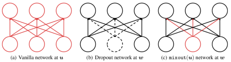
import torch
import torch.nn as nn
import torch.nn.init as init
import torch.nn.functional as F
from torch.nn import Parameter
from torch.autograd.function import InplaceFunction

class Mixout(InplaceFunction):
    @staticmethod
    def _make_noise(input):
        return input.new().resize_as_(input)

    @classmethod
    def forward(cls, ctx, input, target=None, p=0.0, training=False, inplace=False):
        if p < 0 or p > 1:
            raise ValueError("A mix probability of mixout has to be between 0 and 1," " but got {}".format(p))
        if target is not None and input.size() != target.size():
            raise ValueError(
                "A target tensor size must match with a input tensor size {},"
                " but got {}".format(input.size(), target.size())
            )
        ctx.p = p
        ctx.training = training

        if ctx.p == 0 or not ctx.training:
            return input

        if target is None:
            target = cls._make_noise(input)
            target.fill_(0)
        target = target.to(input.device)

        if inplace:
            ctx.mark_dirty(input)
            output = input
        else:
            output = input.clone()

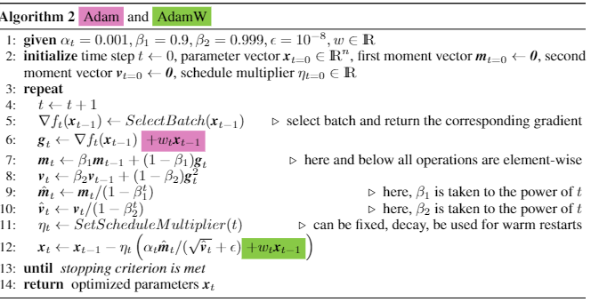
        ctx.noise = cls._make_noise(input)
        if len(ctx.noise.size()) == 1:
            ctx.noise.bernoulli_(1 - ctx.p)
        else:
            ctx.noise[0].bernoulli_(1 - ctx.p)
            ctx.noise = ctx.noise[0].repeat(input.size()[0], 1)
        ctx.noise.expand_as(input)

        if ctx.p == 1:
            output = target
        else:
            output = ((1 - ctx.noise) * target + ctx.noise * output - ctx.p * target) / (1 - ctx.p)
        return output

    @staticmethod
    def backward(ctx, grad_output):
        if ctx.p > 0 and ctx.training:
            return grad_output * ctx.noise, None, None, None, None
        else:
            return grad_output, None, None, None, None


def mixout(input, target=None, p=0.0, training=False, inplace=False):
    return Mixout.apply(input, target, p, training, inplace)


class MixLinear(torch.nn.Module):
    __constants__ = ["bias", "in_features", "out_features"]  # for jit optimization
    def __init__(self, in_features, out_features, bias=True, target=None, p=0.0):
        super(MixLinear, self).__init__()
        self.in_features = in_features
        self.out_features = out_features
        self.weight = Parameter(torch.Tensor(out_features, in_features))
        if bias:
            self.bias = Parameter(torch.Tensor(out_features))
        else:
            self.register_parameter("bias", None)
        self.reset_parameters()
        self.target = target
        self.p = p

    def reset_parameters(self):
        init.kaiming_uniform_(self.weight, a=math.sqrt(5))
        if self.bias is not None:
            fan_in, _ = init._calculate_fan_in_and_fan_out(self.weight)
            bound = 1 / math.sqrt(fan_in)
            init.uniform_(self.bias, -bound, bound)

    def forward(self, input):
        return F.linear(input, mixout(self.weight, self.target, self.p, self.training), self.bias)

    def extra_repr(self):
        type = "drop" if self.target is None else "mix"
        return "{}={}, in_features={}, out_features={}, bias={}".format(
            type + "out", self.p, self.in_features, self.out_features, self.bias is not None
        )

使用：

if mixout > 0:
    print('Initializing Mixout Regularization')
    for sup_module in model.modules():
        for name, module in sup_module.named_children():
            if isinstance(module, nn.Dropout):
                module.p = 0.0
            if isinstance(module, nn.Linear):
                target_state_dict = module.state_dict()
                bias = True if module.bias is not None else False
                new_module = MixLinear(
                    module.in_features, module.out_features, bias, target_state_dict["weight"], mixout
                )
                new_module.load_state_dict(target_state_dict)
                setattr(sup_module, name, new_module)
    print('Done.!')

Mixout相当于一种自适应的 L2-regularizer ，使得参数变化不会很剧烈。能够提高finetuning稳定性。

Pre-trained Weight Decay

将 weight decay 中，gradient减去的 \(\lambda w\) 变为 \(\lambda (w - w^{pretrained})\)。在Mixout文章中，实验表明这样比普通的 weight decay ，finetuning更稳定。

class PriorWD(Optimizer):
    def __init__(self, optim, use_prior_wd=False, exclude_last_group=True):
        super(PriorWD, self).__init__(optim.param_groups, optim.defaults)
        self.param_groups = optim.param_groups
        self.optim = optim
        self.use_prior_wd = use_prior_wd
        self.exclude_last_group = exclude_last_group
        self.weight_decay_by_group = []
        for i, group in enumerate(self.param_groups):
            self.weight_decay_by_group.append(group["weight_decay"])
            group["weight_decay"] = 0
		
        # w pretrained
        self.prior_params = {}
        for i, group in enumerate(self.param_groups):
            for p in group["params"]:
                self.prior_params[id(p)] = p.detach().clone()

    def step(self, closure=None):
        if self.use_prior_wd:
            for i, group in enumerate(self.param_groups):
                for p in group["params"]:
                    if self.exclude_last_group and i == len(self.param_groups):
                        p.data.add_(-group["lr"] * self.weight_decay_by_group[i], p.data)
                    else:
                        # w - w pretrained
                        p.data.add_(
                            -group["lr"] * self.weight_decay_by_group[i], p.data - self.prior_params[id(p)],
                        )
        loss = self.optim.step(closure)

        return loss

    def compute_distance_to_prior(self, param):
        assert id(param) in self.prior_params, "parameter not in PriorWD optimizer"
        return (param.data - self.prior_params[id(param)]).pow(2).sum().sqrt()

使用:

optimizer_grouped_parameters = get_optimizer_grouped_parameters(model, learning_rate, weight_decay)
optimizer = AdamW(
    optimizer_grouped_parameters,
    lr=learning_rate,
    eps=adam_epsilon,
    correct_bias=not use_bertadam
)

# 修改 optimizer
optimizer = PriorWD(optimizer, use_prior_wd=use_prior_wd)

Training Strategies

提升模型速度或准确性的方法：

• Stochastic Weight Averaging
• MADGRAD Optimizer
• Differential / Discriminative Learning Rate
• Dynamic Padding and Uniform Length Batching
• Gradient Accumulation
• Freeze Embedding
• Numeric Precision Reduction
• Gradient Checkpointing

Stochastic Weight Averaging

1. learning rate schedule经过设计，使得模型在“最优解”附近徘徊，而不是收敛到一点（理论上）。比如75%的时间使用standard decaying learning rate strategy ；而剩下的训练在一个相对较高的constant learning rate上训练。

2. 计算训练最后阶段的滑动平均作为SWA的权重

3. SWA权重在训练时，不参与计算。计算Batch Normalization的activation statistics时，在训练结束后，单独进行一次 forward pass 得到activation statistics。

所以，有两组权重，一组训练BP，一组计算保存SWA权重。

示例

from torch.optim.swa_utils import AveragedModel, SWALR
from torch.optim.lr_scheduler import CosineAnnealingLR

loader, optimizer, model, loss_fn = ...
swa_start = 5
swa_model = AveragedModel(model)
swa_scheduler = SWALR(optimizer, swa_lr=0.05)
scheduler = CosineAnnealingLR(optimizer, T_max=100)

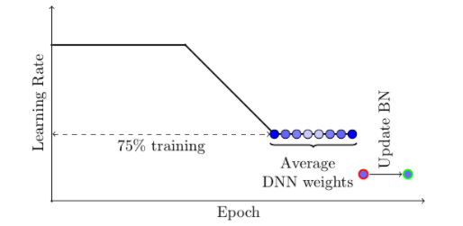
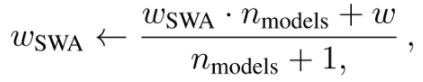
for epoch in range(100):
      for input, target in loader:
          optimizer.zero_grad()
          loss_fn(model(input), target).backward()
          optimizer.step()
      if epoch > swa_start:
          swa_model.update_parameters(model)
          swa_scheduler.step()
      else:
          scheduler.step()

# Update bn statistics for the swa_model at the end
torch.optim.swa_utils.update_bn(loader, swa_model)
# Use swa_model to make predictions on test data 
preds = swa_model(test_input)

refernce

MADGRAD Optimizer

AdaGrad派生出的新优化器，在以下任务中表现较好，包括视觉中的分类和图像到图像的任务，以及自然语言处理中的循环和双向掩蔽模型。

但是，weight decay不同于其他，常常设置为0。 learning rate 的设置也和SGD与Adam不同，必要时，先进行一次learning rate查找。

paper

pip -q install madgrad

另外小数据集上的训练，可以尝试使用RAdam + Lookahead而不是AdamW，效果可能会更好，因为AdamW的warm-up阶段受到数据集大小size的影响。

Differential / Discriminative Learning Rate

模型底层为普遍的字词信息，越往上得到与任务相关的抽象信息。所以 fine-tune 时，对通用层设置较小学习率，越往上学习率相对更大。自定义层学习率单独设置，一般较大。

def get_optimizer_params(model, type='unified'):
    # differential learning rate and weight decay
    param_optimizer = list(model.named_parameters())
    learning_rate = 5e-5
    no_decay = ['bias', 'gamma', 'beta']
    if type == 'unified':
        optimizer_parameters = filter(lambda x: x.requires_grad, model.parameters())
    elif type == 'module_wise':
        optimizer_parameters = [
            {'params': [p for n, p in model.roberta.named_parameters() if not any(nd in n for nd in no_decay)],
             'weight_decay_rate': 0.01},
            {'params': [p for n, p in model.roberta.named_parameters() if any(nd in n for nd in no_decay)],
             'weight_decay_rate': 0.0},
            {'params': [p for n, p in model.named_parameters() if "roberta" not in n],
             'lr': 1e-3,
             'weight_decay_rate':0.01}
        ]
    elif type == 'layer_wise':
        group1=['layer.0.','layer.1.','layer.2.','layer.3.']
        group2=['layer.4.','layer.5.','layer.6.','layer.7.']    
        group3=['layer.8.','layer.9.','layer.10.','layer.11.']
        group_all=['layer.0.','layer.1.','layer.2.','layer.3.','layer.4.','layer.5.','layer.6.','layer.7.','layer.8.','layer.9.','layer.10.','layer.11.']
        optimizer_parameters = [
            {'params': [p for n, p in model.roberta.named_parameters() if not any(nd in n for nd in no_decay) and not any(nd in n for nd in group_all)],'weight_decay_rate': 0.01},
            {'params': [p for n, p in model.roberta.named_parameters() if not any(nd in n for nd in no_decay) and any(nd in n for nd in group1)],'weight_decay_rate': 0.01, 'lr': learning_rate/2.6},
            {'params': [p for n, p in model.roberta.named_parameters() if not any(nd in n for nd in no_decay) and any(nd in n for nd in group2)],'weight_decay_rate': 0.01, 'lr': learning_rate},
            {'params': [p for n, p in model.roberta.named_parameters() if not any(nd in n for nd in no_decay) and any(nd in n for nd in group3)],'weight_decay_rate': 0.01, 'lr': learning_rate*2.6},
            {'params': [p for n, p in model.roberta.named_parameters() if any(nd in n for nd in no_decay) and not any(nd in n for nd in group_all)],'weight_decay_rate': 0.0},
            {'params': [p for n, p in model.roberta.named_parameters() if any(nd in n for nd in no_decay) and any(nd in n for nd in group1)],'weight_decay_rate': 0.0, 'lr': learning_rate/2.6},
            {'params': [p for n, p in model.roberta.named_parameters() if any(nd in n for nd in no_decay) and any(nd in n for nd in group2)],'weight_decay_rate': 0.0, 'lr': learning_rate},
            {'params': [p for n, p in model.roberta.named_parameters() if any(nd in n for nd in no_decay) and any(nd in n for nd in group3)],'weight_decay_rate': 0.0, 'lr': learning_rate*2.6},
            {'params': [p for n, p in model.named_parameters() if "roberta" not in n], 'lr':1e-3, "momentum" : 0.99},
        ]
    return optimizer_parameters

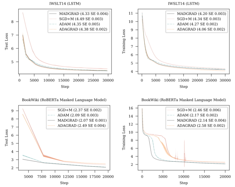
Strategies: 对于小数据集，复杂的learning rate scheduling strategies（linear with warmup or cosine with warmup etc.）在预训练和finetuning阶段都没什么效果。小数据集，使用简单的scheduling strategies就行。

from transformers import (  
    get_constant_schedule, 
    get_constant_schedule_with_warmup, 
    get_cosine_schedule_with_warmup, 
    get_cosine_with_hard_restarts_schedule_with_warmup,
    get_linear_schedule_with_warmup,
    get_polynomial_decay_schedule_with_warmup
)

Interpreting Transformers with LIT

transfomer可视化工具

Paper: The Language Interpretability Tool: Extensible, Interactive Visualizations and Analysis for NLP Models Blog: The Language Interpretability Tool (LIT): Interactive Exploration and Analysis of NLP Models Official Page: Language Interpretability Tool Examples: GitHub

Dynamic Padding and Uniform Length Batching

常规padding策略如上图所示，pad到最大长度。

Dynamic Padding就是每个batch，分别pad到该batch中最长的序列长度。

而Uniform Length Batching，则是将长度相近的序列组合成一个batch。

示例程序

import random
import numpy as np
import multiprocessing
import more_itertools

import torch
import torch.nn as nn
from torch.utils.data import Sampler, Dataset, DataLoader

class SmartBatchingDataset(Dataset):
    “tokenize并得到dataloader”
    def __init__(self, df, tokenizer):
        super(SmartBatchingDataset, self).__init__()
        # 这里 df.excerpt 表示dataframe中的文本所在列，使用时需要替换
        self._data = (
            f"{tokenizer.bos_token} " + df.excerpt + f" {tokenizer.eos_token}" 
        	).apply(tokenizer.tokenize).apply(tokenizer.convert_tokens_to_ids).to_list()
        self._targets = None
        if 'target' in df.columns:
            self._targets = df.target.tolist()
        self.sampler = None

    def __len__(self):
        return len(self._data)

    def __getitem__(self, item):
        if self._targets is not None:
            return self._data[item], self._targets[item]
        else:
            return self._data[item]

    def get_dataloader(self, batch_size, max_len, pad_id):
        self.sampler = SmartBatchingSampler(
            data_source=self._data,
            batch_size=batch_size
        )
        collate_fn = SmartBatchingCollate(
            targets=self._targets,
            max_length=max_len,
            pad_token_id=pad_id
        )
        dataloader = DataLoader(
            dataset=self,
            batch_size=batch_size,
            sampler=self.sampler,
            collate_fn=collate_fn,
            num_workers=(multiprocessing.cpu_count()-1),
            pin_memory=True
        )
        return dataloader
    
    
class SmartBatchingSampler(Sampler):
    “按序列长度排序，得到一组shuffle之后的batch data”
    def __init__(self, data_source, batch_size):
        super(SmartBatchingSampler, self).__init__(data_source)
        self.len = len(data_source)
        sample_lengths = [len(seq) for seq in data_source]
        argsort_inds = np.argsort(sample_lengths)
        self.batches = list(more_itertools.chunked(argsort_inds, n=batch_size))
        self._backsort_inds = None
    
    def __iter__(self):
        if self.batches:
            last_batch = self.batches.pop(-1)
            np.random.shuffle(self.batches)
            self.batches.append(last_batch)
        self._inds = list(more_itertools.flatten(self.batches))
        yield from self._inds

    def __len__(self):
        return self.len
    
    @property
    def backsort_inds(self):
        “未shuffle时，batch序列按照长度排序的结果”
        if self._backsort_inds is None:
            self._backsort_inds = np.argsort(self._inds)
        return self._backsort_inds
    
class SmartBatchingCollate:
    “每个batch分别pad到最大长度，得到attention mask，处理target”
    def __init__(self, targets, max_length, pad_token_id):
        self._targets = targets
        self._max_length = max_length
        self._pad_token_id = pad_token_id
        
    def __call__(self, batch):
        if self._targets is not None:
            sequences, targets = list(zip(*batch))
        else:
            sequences = list(batch)
        
        input_ids, attention_mask = self.pad_sequence(
            sequences,
            max_sequence_length=self._max_length,
            pad_token_id=self._pad_token_id
        )
        
        if self._targets is not None:
            output = input_ids, attention_mask, torch.tensor(targets)
        else:
            output = input_ids, attention_mask
        return output
    
    def pad_sequence(self, sequence_batch, max_sequence_length, pad_token_id):
        max_batch_len = max(len(sequence) for sequence in sequence_batch)
        max_len = min(max_batch_len, max_sequence_length)
        padded_sequences, attention_masks = [[] for i in range(2)]
        attend, no_attend = 1, 0
        for sequence in sequence_batch:
            # 限制model所允许的最大长度
            new_sequence = list(sequence[:max_len])
            
            attention_mask = [attend] * len(new_sequence)
            pad_length = max_len - len(new_sequence)
            
            new_sequence.extend([pad_token_id] * pad_length)
            attention_mask.extend([no_attend] * pad_length)
            
            padded_sequences.append(new_sequence)
            attention_masks.append(attention_mask)
        
        padded_sequences = torch.tensor(padded_sequences)
        attention_masks = torch.tensor(attention_masks)
        return padded_sequences, attention_masks

使用：

dataset = SmartBatchingDataset(train, tokenizer)
dataloader = dataset.get_dataloader(batch_size=24, max_len=max_len, pad_id=tokenizer.pad_token_id)

已经证明，这种技术不仅显著的减少了训练时间，而且不会减少准确性（在某些情况下甚至提高）。

Freeze Embedding

Freezing Embedding Layer of transformers加速训练并节省显存。

一种解释是（看看就好，没有严格证明）：finetuning用的小数据集中，新出现的token会导致原language model中学习好的局部同义词间结构关系被破坏。

import transformers
from transformers import AutoConfig, AutoModelForSequenceClassification

freeze_embedding = True

config = AutoConfig.from_pretrained('roberta-base')
model = AutoModelForSequenceClassification.from_pretrained(
    _pretrained_model, config=config
)
model.base_model.embeddings.requires_grad_(not freeze_embedding)

这种方法，可以一试，可以用更大的batch size。

Numeric Precision Reduction

混合精度。常见的推理加速方法。

在过去的几年，GPU硬件对float16操作的糟糕支持，意味着降低权重和激活值的精度通常会适得其反，但是NVIDIA Volta和Turing架构与张量核心的引入，意味着现代GPU可以更高效的支持float16运算。

大多数transformer网络都可以简单地转换为float16权值和激活值计算，而没有精度损失。

之所以要保留float32，是因为像softmax这类，计算时有较长的连加运算，这时使用float16可能存在精度损失。

半精度的加速来源于，半精度计算指令本身的速度更快，另外此时可以使用更大的batch size。

开源工具：NVIDIA-apex；torch.cuda.amp--相比AMP，使用更灵活一些，但是用起来都差不多。

注意：小batch size时，混合精度会由于频繁IO导致的时间损失大于小batch的半精度训练所节省的时间。

示例

Gradient Accumulation

就是累计梯度几个轮次，然后进行一次参数更新。

示例程序

optimizer.zero_grad()                               # Reset gradients tensors
for i, (inputs, labels) in enumerate(training_set):
    predictions = model(inputs)                     # Forward pass
    loss = loss_function(predictions, labels)       # Compute loss function
    loss = loss / accumulation_steps                # Normalize our loss (if averaged)
    loss.backward()                                 # Backward pass
    if (i+1) % accumulation_steps == 0:             # Wait for several backward steps
        optimizer.step()                            # Now we can do an optimizer step
        optimizer.zero_grad()                           # Reset gradients tensors
        if (i+1) % evaluation_steps == 0:           # Evaluate the model when we...
            evaluate_model()                        # ...have no gradients accumulated

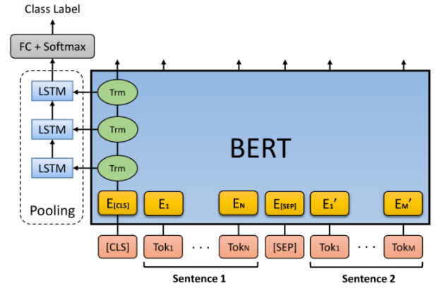
如果我们的损失是在训练样本上平均的，我们还需要除以积累步骤的数量。

Gradient Checkpointing

以时间为代价，节省GPU内存。

通过将模型分为不同的段，每个段计算时，分别进行计算，将当前段计算结果传给下一个段后，当前段的中间状态都不会保存。

示例 PyTorch Checkpoint多GPU优化

其他开源工具

• DeepSpeed
  
• FairScale
• Accelerate

Some Exp

1. 讲实话小样集的比赛，是个调参游戏，对于回归任务，更是如此。结构上玩出花，效果反而不好。优化方法上，常见的FGM和SWA对于一些回归任务，基本没啥效果提升。没有尝试过对比学习，可能这是一个好方法。
2. 比赛中对于这类强学习模型，还是最好bagging，降降variance。
3. 只把BERT这些庞然大物当做特征抽取器，然后用传统ML算法来学习，会是更方便快捷的方法，而且实践上也确实可行，只是很容易过拟合，BERT特征还是太强了（当然这取决于如何训练和训练的程度）。这可能更快，但是得到好结果需要一些“运气”，还有一点直觉。
4. 对于比赛而言，large模型得到好结果还是容易一些，就像好多论文，其实方法就那样，主要BERT 类模型用large调得好，也容易出好结果。可解释的余地还是太差了。各部分又几乎是关联的，耦合在一起，所以算了。
5. 好的算法，不应该是亿级参数对数据的变相记忆，那是“数据库”的加权求和与激活函数筛选。让人感觉失望。这里的一面之词是，大模型，总是“不太好”。可是，效果有了，很多时候，还是会真香。

NLP Tutorial

• The Super Duper NLP Repo
• Huggingface Community
• Hugging Face’s notebooks

reference：

• kaggle rhtsingh
• REVISITING FEW-SAMPLE BERT FINE-TUNING
• ON THE STABILITY OF FINE-TUNING BERT
• SMART: Robust and Efficient Fine-Tuning for Pre-trained Natural Language Models
• Fine-Tuning Pretrained Language Models:Weight Initializations, Data Orders, and Early Stopping
• MIXOUT: EFFECTIVE REGULARIZATION TO FINETUNE LARGE-SCALE PRETRAINED LANGUAGE MODELS
• How to Fine-Tune BERT for Text Classification?
• Sentence Encoders on STILTs: Supplementary Training on Intermediate Labeled-data Tasks